Power electronics are an essential subsystem within the architecture of an electric vehicle. Their performance has a direct influence on the torque provided by an electric motor. In turn, this impacts electric vehicle performance, such as acceleration. What’s more, power conversion always generates heat, and this increases the temperature of the semi-conductors. If this rise in temperature is not controlled, the semi-conductors will be at risk of failure.
Typical power electronics include AC/DC converters (rectifiers), DC/DC converters (choppers), DC/AC converters (inverters), AC/AC converters (gradators), which are all built with inductors, capacitors, semiconductors and transformers.
With Simcenter Amesim, engineers can accurately simulate performance of electric vehicle components and systems, including thermal analysis. In addition, the Simcenter Amesim model can be linked to Simulink for real-time simulations, including hardware-in-the-loop testing.
In this post, we explore some examples demonstrating how Simcenter Amesim can help you design power electronics devices.
First off, Simcenter Amesim offers a dedicated off-the shelf library for a given physical domain of interest, which is very useful. In the case of power electronics, this is the Electrical Static Conversion library (Fig. 1).
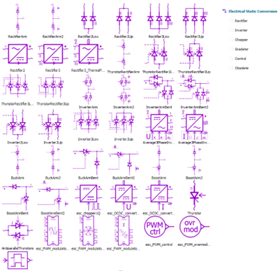
Fig. 1 Content of Electrical Static Conversion Library
Switched Reluctance Motor Control
Precise control of power semi-conductors is required for Switched Reluctance Motors to work with high efficiency and low torque ripple. Optimizing power electronics control is a complex task, and simulations are widely used to shorten the control algorithm development time. Developing electric motor control on a “live system” is slow, costly and risky.
The first example presents a high-speed control of a three-phase 6/4 (6 poles on the stator, 4 on the rotor) switched reluctance motor.
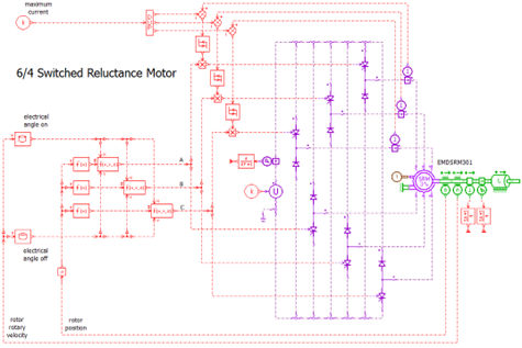
Fig. 2 Maximum current control on a 6/4 switch reluctance machine
In this control application, the three-phase currents are controlled independently. Depending on the rotor position, phase A, B and C currents are regulated to a constant maximum value or to zero, thanks to a hysteresis control. The converter will then apply a variable voltage to the machine phases (Fig. 3).
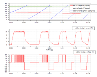
Fig. 3 SRM phase A current and voltage control (low speed)
To get the highest possible mechanical power and efficiency at a given speed, the rotor position where the current starts to be regulated to its maximum value (angle on) and the position where the current starts to be regulated to zero (angle off) have been optimized. They can be very different at low and high speeds, giving a different behavior in both cases. (Fig. 4).
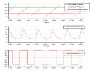
Fig. 4 SRM phase A current and voltage control (high speed)
Thanks to the model of the control logic, the current in this model never reaches its maximum value or zero. The machine is able to provide a torque even for very high speeds with a good efficiency (Fig. 5).
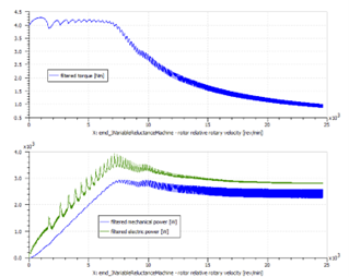
Fig. 5 SRM torque and efficiency results
PWM inverter thermal analysis
While designing power electronics devices, the thermal aspects are also of significant importance. In extreme cases, there is a risk of a thermal runoff, where increases in temperature can lead to higher heat dissipation, which in turn will produce an additional rise in temperature, resulting in overheating and device failure.
To illustrate this, the second example in this blog is a three-phase PWM inverter model with thermal management. In this example, the electric components are connected to thermal models that simulate the thermo-electric feedback seen in semiconductor circuits: the heating of components leads to changes in the electrical behavior, which in turn will change the heating dynamics.
We will investigate how the junction temperature in both the transistor and diode influences their electrical behavior. And in turn, how the electrical behavior will have an impact on the heat generation.
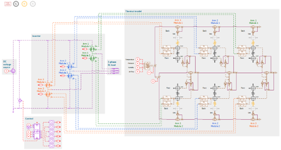
Fig. 6 Thermal model of a PWM 3 phase inverter with thermal management
Semi-conductors characteristics
In this model the PWM signals control three inverter arms that are built with a transistor and an anti-parallel diode, both housed inside a single case known as a module. Therefore, the inverter is made up of six such modules.
The switching losses can be defined as a function of current, voltage and temperature:
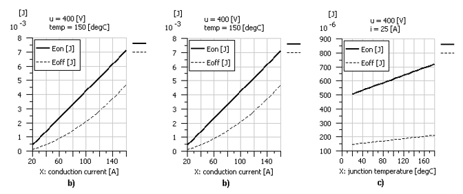
Fig. 7 Switching energy losses as a function of:
a) forward voltage, with current at 25 [A] and temperature to 150°C
b) conduction current, with voltage at 400 [V] and temperature to 150°C
c) junction temperature, with voltage at 400 [V] and current to 25 [A]
To define the characteristic curves shown above, a reference point with junction temperature at 150°C, transistor/diode forward voltage to 400 [V] and conduction current equal to 25 [A] was used; the influence of each parameter is considered separately. That is, the junction temperature plot shows the temperature influence while other values are kept constant; the same thing is then done for current and voltage.
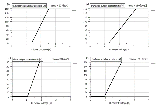
Fig. 8 Conduction characteristics for 2 temperatures values
Both parameters, switching and conduction characteristics, dictate the diode/transistor losses. The heat losses are transferred to a thermal model that returns the temperature of the individual components. This heat flow is also used to calculate the case, sink and ambient temperature.
We will consider two cases: warm-up stage and steady state operation.
Warm-up stage
In the warm-up case, the temperature state variables are initialized to ambient temperature. The inductor current state variables are set to zero. Though the influencing phenomena are difficult to separate at the beginning of the transition, a higher-than-normal current will go through the second phase, creating a higher-than-normal heat flow in the transistor. And, inversely, a lower than normal current in the diode. Because of this, diode heat losses will be smaller during the transition phase.
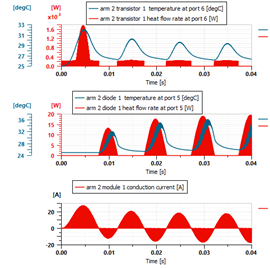
Fig. 9 Module current influence on heat flow rate
It may be important, when sizing the cooling system and optimizing the geometric position of these components, to consider the temperature differences between each component. Even though the simulation covers only a few fractions of a second, these differences are already apparent: figure 10 shows the differences between the three sinks and the surrounding air “chamber” temperatures.
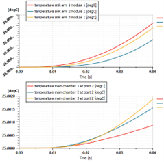
Fig. 10 Temperature differences with position
This difference can also be observed in the animated 3D view where colors vary to illustrate temperature changes. In this case, the main body of the module is hotter than the upper part. The sink is even colder than the body (module) because a larger area is exposed to the cool air.

Fig. 11 3D animation preview in Amesim
In the steady state case, the inverter’s currents and its temperature variations are periodic.
Steady state operation
Now we can compare the heat flow of the same transistor in the initial run and in this new final state. This is shown in figure 12, where the left-hand graph shows a small heat flow at around 25°C. In the right hand graph, the heat flow rate is greater. This is because the component temperature starts at 65°C and because of a higher steady state current.
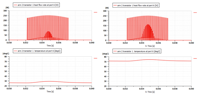
Fig. 12 Temperature influence on heat flow rate
There is also a temperature difference between the different layers of a single module. The diode and transistor each have a different dynamic caused by the different electrical behaviors. The module body temperature is calculated by adding up both heat flows.
Additionally, the temperature differences between the main body, upper body and sink can be perceived. The figure below shows these differences in the second module of all three inverter arms.
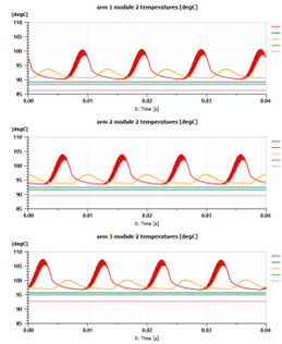
Fig. 13 Temperature and behavior differences by layer (one module from each inverter arm)
In the previous plots, heat flow rates were shown. This flow is made up of switching and conduction losses. The next plot shows both flow types separately. A slight difference in the peak values can be observed because losses increase linearly with temperature. However, the temperature influence is much smaller when compared to the current influence on the semiconductor losses (see figure 7).
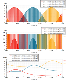
Fig. 14 Transistor losses and temperature influence
Thanks to this advanced modeling of electrical parameters and thermal network, the transistor junction temperature can be accurately modeled. We can see how position affects the final temperature value: the average temperature increases by 5 degrees for each successive module pair. In addition, the actual peak temperature values can be very different from the average value, highlighting the utility of the equivalent thermal impedance model.
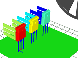
Fig. 15 3D view of the temperature difference between components
In this case, as can be observed in the image above, the first module pair located closest to the air flow rate is kept at a comfortable temperature, at 59°C. The second pair is at around 64°C. And the third component is above 70°C, which is more than a 10°C difference.
Thanks to the approach used, the local air temperature is taken into account when evaluating heat transfers. In addition, the temperature rise of the different materials that make up the exterior of the electrical module (transistor + diode) can be visualized.
Consequently, a better evaluation of each junction’s final temperature is obtained. All of this insight can be paramount during thermal cooling development: instead of implementing large safety margins, because junction temperatures are known, a more constrained approach can be adopted. This gives designers the possibility of implementing a smaller and more economical thermal solution.
How are the power electronics performing and are they thermally happy?
It is paramount for an electric vehicle’s performance that its power electronics be optimized for torque and speed control. Simcenter Amesim provides insight into the behavior of components and systems across complex duty cycles. Engineers can carry out virtual validation and predict any issues, such as “cooking” semi-conductors as a result of the cooling system not being up to scratch.
Get a better handle on the performance of electric vehicle components and systems with Simcenter Amesim.
Ready to get started? Contact a Maya HTT expert today.