
NASA’s new requirements for spacecraft designs
With the introduction of NASA’s new technical standard NASA-STD-5002B for load analyses of spacecraft and payloads, the pre-test step has become a critical part of spacecraft design workflows.
In particular, Section 4.9.1 Pre-Test Analysis introduces a pre-test verification requirement for mass orthogonality checks and self-orthogonality criteria to ensure reduced model accuracy.
Aside from risking non-compliance, companies that cannot meet the new NASA standards will experience less efficient workflows, making them less competitive in the space market.
Space: from exploration to exploitation
The space market has undergone a significant shift from exploration to exploitation. Commercial profitability now drives the space economy, with a focus on reusable technologies, increasingly compressed development cycles, and aggressive price targets – all of which are pushing verification away from physical testing and towards simulation.
What are the implications for spacecraft design?
- Flexible methodologies
- Short development cycles
- Lower prices
Spacecraft structural testing is expensive, schedule-sensitive, and difficult to repeat. By the time hardware reaches the test floor, engineers need to be confident that the planned modal test will generate data that can support meaningful finite element model correlation.
Expertise in the field
At Maya HTT, our expertise includes simulation for spacecraft design. We know what can go wrong and we can help you get testing right.
- A poor sensor layout can lead to weak modal observability, inconclusive correlation, and costly re-test decisions.
- Poor upstream pre-testing practices can mean weeks of launch delays as well as unscheduled program expenses.
Auto-MAC alone cannot ensure an efficient test. A more thorough workflow is needed, and is, in fact, now required by NASA-STD-5002B.
By leveraging state-of-the-art pre-test, correlation, and model update simulation software, you can reduce your risk of costly re-testing and comply with NASA’s latest Spacecraft and Payload Analysis Standard. Our experts are available to help.
A question of pre-test diagnostics
When it comes to pre-test diagnostics, there are four essential concerns:
- Why sensor placement alone is not enough to guarantee a correlation-ready modal test
- How AutoMAC, self-orthogonality, pseudo-orthogonality, and cross-orthogonality each reveal different pre-test risks
- What failing orthogonality metrics suggest about sensor layout, reduced mass representation, and modal basis quality
- How to use pre-test diagnostics to improve instrumentation plans before hardware reaches the test floor
Pre-test mass-orthogonality checks are critical because a modal test does not observe the full finite element model. It observes the structure only through the selected sensor degrees of freedom.
A sensor layout may seem reasonable, geometrically, and it may even produce an acceptable AutoMAC matrix, but that does not mean the selected test degrees of freedom preserve the independence of the target modes when evaluated through the reduced mass matrix.
Pre-test validation answers another, more important question: Will this planned modal test provide data that can support reliable model correlation?
From sensor placement to test readiness
To explore that question, let’s explore the following example of a spacecraft antenna.
The workflow begins with a finite element modal survey. In this example, the test article is a spacecraft antenna subcomponent modeled using Simcenter NASTRAN. A Simcenter NASTRAN normal modes analysis extracts the first twenty target modes.
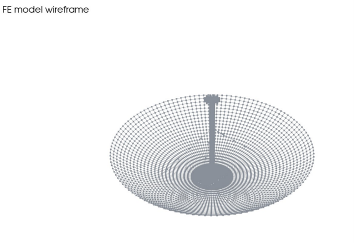
Fig 1: Sample wireframe view of the antenna model.
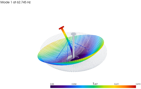
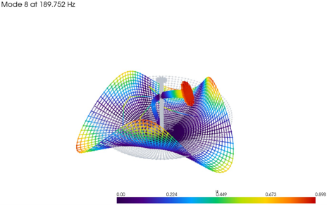
Fig 2: Sample modes (1 and 8) of the antenna model.
A modal survey shows effective mass participation distributed across the three translational directions.
The test plan sensors must distinguish the target modes and provide sufficient modal observability. Otherwise, the result will be limited test coverage, leading to low correlation between the actual model and the digital model, as shown in the table below.
| Mode | frequency_hz | eff_mass_x_percent | eff_mass_y_percent | eff_mass_z_percent | eff_mass_percent |
| 1 | 62.7 | 0.0004 | 2.08 | 2.94 | 5.02 |
| 2 | 77.7 | 2.08 | 0.0002 | 2.94 | 5.02 |
| 3 | 96.5 | 0.59 | 0.54 | 3.85 | 4.98 |
| 4 | 135.5 | 0.42 | 1.2 | 3.32 | 5.00 |
| 5 | 135.7 | 0.23 | 2.67 | 2.15 | 5.05 |
| … | |||||
| 15 | 250.7 | 1.78 | 0.34 | 2.85 | 4.98 |
| 16 | 251.0 | 1.65 | 0.47 | 2.85 | 4.98 |
| 17 | 300.6 | 0.74 | 0.71 | 3.52 | 4.98 |
| 18 | 301.5 | 0.77 | 0.70 | 3.50 | 4.98 |
| 19 | 314.1 | 2.48 | 2.47 | 0.02 | 4.98 |
| 20 | 344.6 | 0.078 | 0.04 | 4.86 | 4.98 |

Table 1: Effective mass participation.
Next, several sensor-placement are evaluated for a target set of forty uniaxial sensors.
|
Min-MAC & MODMAC |
Can the sensors distinguish one mode from another? |
|
Min-MAC and MODMAC |
Can the sensors distinguish one mode from another? |
|
Effective independence with the fisher information matrix |
Can the sensors provide enough independent information to estimate the target modal basis? |
|
Modal kinetic energy |
Are the sensors located where the structure actually moves? |
|
Information entropy index |
Is there a balance between response strength and broad modal coverage? |
Table 2: Sensor-placement.
In our antenna example, Min-MAC and MODMAC provide the best modal discrimination.
Here, the Min-MAC sensor set is selected for mass-orthogonality validation. None of these methods directly target the matrix that matters for mass orthogonality. A new method to directly target mass orthogonality is out of the scope of this article.
Why AutoMAC is not enough
A clean AutoMAC matrix is valuable, but it is not the end of pre-test validation. AutoMAC shows whether the target modes appear distinguishable through the selected sensor degrees of freedom. However, it does not fully prove that the reduced mass operator and retained test degrees of freedom preserve modal independence for correlation.
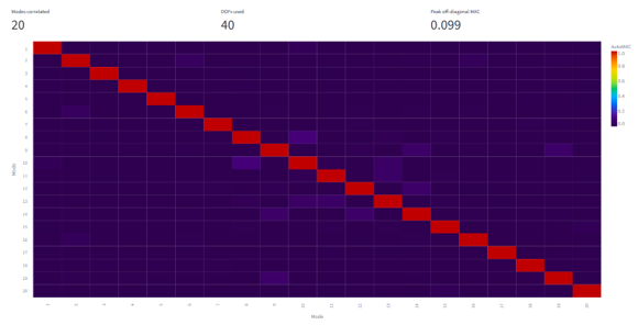
Fig 3: AutoMAC matrix for MIN-MAC method for sensor prediction DOFs.
It is at this point that mass-orthogonality validation becomes essential.
The NASA-STD-5002B-style target is an identity-like orthogonality matrix. Diagonal terms should be close to one, and off-diagonal terms should be small. Low off-diagonal terms mean the modes remain distinct. Large off-diagonal values indicate mode coupling or ambiguity. Weak diagonal values indicate that a mode is poorly represented by the selected degrees of freedom.
Three complementary checks are used: self-orthogonality, pseudo-orthogonality, and cross-orthogonality.
|
Metric |
Possible reason for failure |
What to inspect or change |
|
Self-orthogonality |
Selected sensor DOFs do not preserve modal independence well enough, or the reduced analytical mass matrix does not represent the retained test DOFs accurately. |
Sensor placement, modal observability at the chosen DOFs, Guyan reduction setup, retained DOF definition, and reduced mass matrix extraction. |
|
Pseudo-orthogonality |
Reduced A-set modal basis is not properly mass-normalized or the retained-DOF reduction introduces inconsistency in the reduced modes. |
A-set extraction, reduced eigenvector generation, mass normalization, retained DOF mapping, and reduced model assembly. |
|
Cross-orthogonality |
Reduced basis does not represent the same physical modes as the unreduced FEM cleanly, often due to mode pairing errors, mode mixing, or insufficient capture of coupled modes. |
Mode pairing, closely spaced modes, sensor coverage near modal anti-nodes, retained DOF selection, and regenerate or refine the reduced modal basis. |
Table 3. Evaluation of complementary checks.
This final check is especially important because it can expose mode pairing issues, mode mixing, or reduction mismatches that are not evident from AutoMAC alone.
In the antenna example, cross-orthogonality fails the target criteria. The matrix indicates that some modes are not represented cleanly by the selected sensor set and reduced modal basis. Closely spaced or coupled modes may require additional sensors, repositioned sensors, or changes to the retained DOF set, all leading to delays and extra test costs.
This is the key value of the workflow: it identifies a test-correlation risk before the modal test is performed.
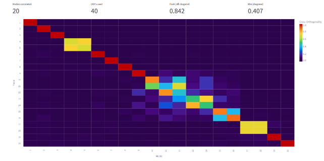
Fig 4: Cross orthogonality matrix. Cross-orthogonality red flag: peak |off-diagonal| 0.842 at modes 12 / 11 exceeds 0.20; minimum |diagonal| 0.407 at mode 11 is below 0.80.
Actionable diagnostics for engineers
The result is not just “pass” or “fail.” The workflow described provides actionable diagnostics needed to set the stage for success.
In the antenna example, the practical recommendation is to add or reposition sensors near the anti-nodes of weakly represented modes, improve the capture of closely spaced mode pairs, regenerate the reduced basis, and repeat the orthogonality checks before releasing the test plan.
How to comply with NASA-STD-5002B
A successful modal test begins before the test article reaches the lab. It begins with a validated sensor layout, a trustworthy reduced mass matrix, and unmistakable evidence that the selected test degrees of freedom can preserve the modes that matter. Poor sensor layouts often lead to inconclusive test and costly re-test decisions, adding delays to the program.
The method presented here is a proven pre-test modal validation method compliant with NASA Standards.
The antenna example shows why mass orthogonality matters: Although a Min-MAC-based sensor set produced strong modal discrimination and passed self- and pseudo-orthogonality checks, cross-orthogonality revealed mode mixing and weak modal representation that must be addressed before test.
Section 4.9.1 was added to NASA-STD-5002B to catch reduced-model/mass-matrix and mode-shape problems before time is spent on modal testing, and to ensure the reduced model is accurate enough for later test-analysis correlation and loads prediction.
Ready to explore how you can reduce testing risk, duration, and cost? Take the first step to avoid the costly pitfall of re-testing without planning.