The McGill Formula Electric team designs, manufactures, and races a Formula-style electric vehicle every year. In part one of this blog series, the cooling system of the vehicle was created in Simcenter Amesim to validate that cooling requirements could be met by the current design. The geometry was represented by macro parameters in Amesim. If you missed it, you can read all about it here.
In part two, we look at how computational fluid dynamics (CFD) can be used to validate and enhance the accuracy of an Amesim model.
Problem statement
CFD simulation is critical in the design of any cooling system components. It makes it possible to go beyond the empirical relations a software like Amesim uses to compute pressure drops and heat fluxes. The geometries for the motor cooling jacket, the inverter cold plate, and the battery pack were simulated in Star-CCM+ to characterize their steady state and transient cooling performance under different conditions.
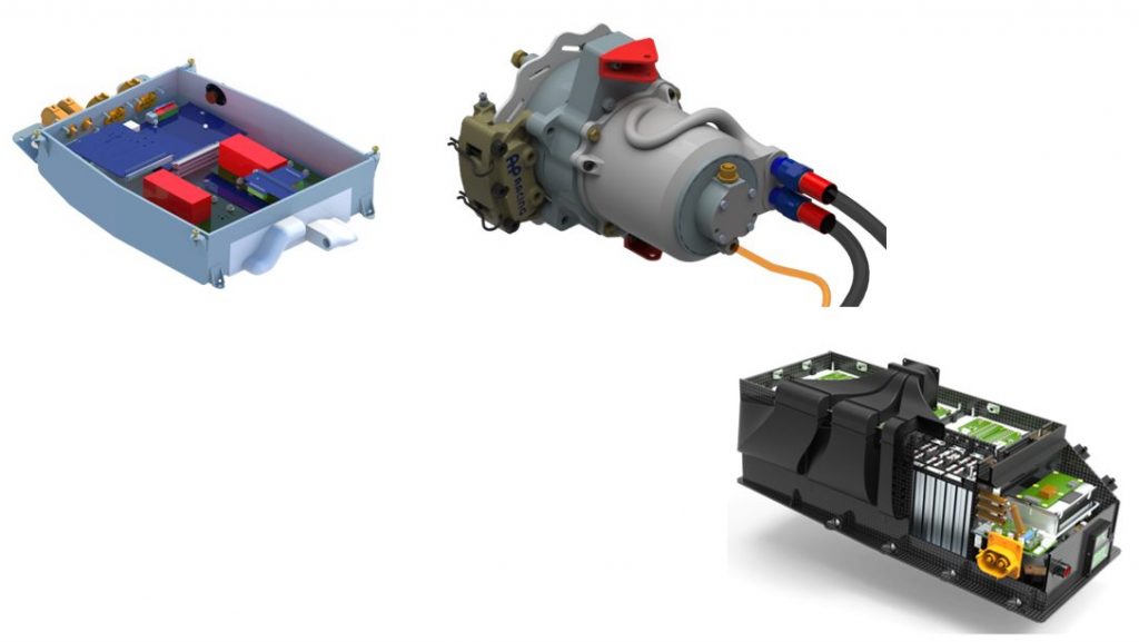
Figure 1-3: Inverter, motor, and battery pack assembly
Liquid cooling
The simulation for the inverter’s cold plate and for the motor cooling jacket used the same continua and set up. In both cases, the geometry was simplified and the assumption that all the heat generated is absorbed by the coolant was kept. This enables a comparison of results with the Amesim model.
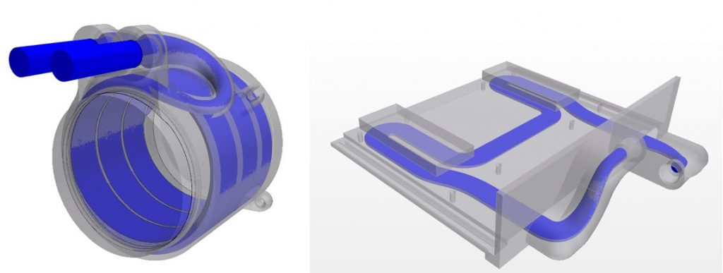
Figure 4-5 Simulation domain for the cooling jacket and the cold plate
The coolant was meshed with a low-y+ approach to ensure good accuracy of the heat transfer at the fluid-wall interfaces. The motor and the inverter heat sinks were approximated as simple shapes with volumetric heating. The heat generation values were those obtained from taking the steady-state heat flux from the Amesim model. Lastly, inlet coolant temperatures and coolant flow rate were set to match those of the Amesim model as well.
Table 1: Amesim and Star CCM+ result comparison
| Cold Plate | Cooling Jacket | |||
| Amesim | Star-CCM+ | Amesim | Star-CCM+ | |
| Heat Absorption (W) | 110/inverter | 800/motor | ||
| Water Temperature Increase (⁰C) | 0.3 | 0.3 | 1.3 | 1.3 |
| Average Device temperature (⁰C) | 31.1 | 30.6 | 36.6 | 35.3
|
The temperature increase is consistent across CFD and Amesim, as it should be, since we are assuming that all the heat is absorbed by the coolant. This value can also be worked out using paper and pen with the coolant mass flow rate, coolant properties, and heat absorption. It is consistent across software and theory.
There is, however, a difference for the average temperature of the individual components. For the cold plate, most of the heat transfer occurs at the interface between the heat sinks and the cold plate. The geometry of the coolant channel was designed to maximize heat transfer in these two zones. The discretization of the domain is critical in that case to resolve this local heat transfer.
A similar argument can be made for the cooling jacket. The Amesim model was not tuned to account for these localized effects, hence the discrepancy. The bends and intricacies of the geometry were also not accounted for in Amesim. These features induce more turbulence in the flow, which also enhances heat transfer.
Figure 6-7 Temperature streamlines
Transient response of the cooling devices
One assumption of the Amesim model is that all the heat must go through the lump mass of metal representing the electric components. This introduces a delay between the heat rejection from the device and the heat absorption from the coolant. The validity of this assumption was also tested by running a transient simulation of the cooling jacket to compare the thermal time response in Star-CCM+ to the one in Amesim. Both curves correspond to the response to a step input in heat generation at time zero.
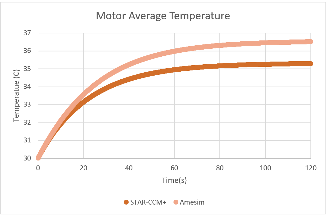
Figure 8: Time response of the motor temperature in Star-CCM+ and Amesim
The time constant τ=0.632*∆T for the CFD simulation and 25s for the system simulation. The rate of change of temperature is initially the same, but as it was discovered in the steady state simulation, the CFD simulation stabilizes to a lower temperature, and it will do so faster. This discrepancy could be corrected many ways in Amesim: by tweaking the parameters, creating a reduced-order-model, or going for co-simulation.
Battery pack air cooling with Star-CCM+
The simulation of the battery pack is more involved: it requires more geometry and the electrical behavior of the system also needs to be modelled. The pack is split into six modules with one cooling fan per module. One of these modules was simulated in Star-CCM+.
The CAD of the battery pack was simplified and imported into Star-CCM+. The box in which each module is enclosed was also imported and used to extract the air volume. The flow enters on the right side and leaves at a 90-degree angle at the bottom.
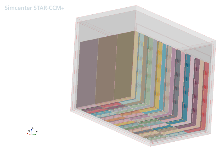
Figure 9: Simplified module geometry with the box and the battery cells
A mass flow inlet with a pressure outlet were created to simulate the airflow through the pack. An RCR model was created for the battery cells using a fitting tool along with test data from a hybrid pulse power characterization test (HPPC) and imported into STAR-CCM+. The electrical load case was exported from the Amesim model.
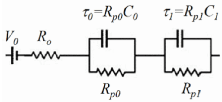
Figure 10: Equivalent RCR circuit for a battery cell
At the time of writing this post, the simulation set-up is complete, but the analysis work remains. This analysis will allow us to validate what combination of mass flow rate of air, battery cell configuration, and load case ensures that all battery cells remain within their specified operating temperatures.
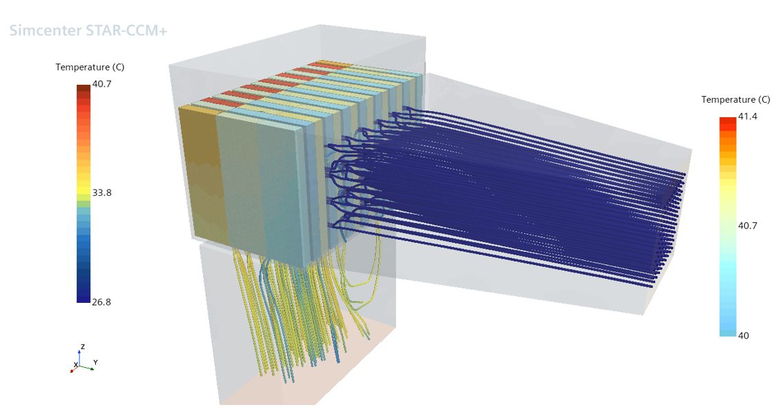
Figure 11: Cell temperature and air temperature streamlines
Star-CCM+ is the tool of choice to perform this analysis, as it allows us to get localized data and individually monitor each cell.
Next steps and conclusion
Obtaining CFD results is a must for the design of any cooling device. This has been done here in parallel to the systems’ simulation, and both results were compared. Some level of discrepancy was found between the two approaches. This was expected. It’s important to reiterate that both analysis methods have their place in the design process. These gaps will be addressed in the next post by leveraging the CFD data to improve the system simulation. This will allow us to bring the best of both worlds together to produce an accurate and comprehensive digital twin of the cooling loop.