How to map flow forces to a structural analysis in Simcenter

Quick Overview

Simcenter offers a dedicated application to map steady state or transient flow results onto a target model, typically an independent structural model from the same geometry but with a different mesh. For example, one could be interested in the stress and distortion analysis of a canopy due to wind forces.

The target FEM must use the same global coordinate system as the source FEM, and both models should be geometrically congruent. However, they need not share the same mesh. Results are mapped from the selected solution on the source model, to a solution on the target model, based on proximity and with optional zone associations. The output of the mapping solution can then be used by the target solution.

In what follows, we describe how to create an NX Nastran structural analysis using forces that are mapped from a Simcenter Thermal/Flow analysis.

Workflow overview

The main steps are:

1. Create a part file containing the structure and air volume.
2. Create a Simcenter Thermal/Flow fem file with only the air volume meshed.
3. Create a new Simulation containing a Thermal/Flow Solution with Flow Analysis.
4. Run the Thermal/Flow Solution.
5. Back to the part file; create a NX Nastran fem file of the structure.
6. Create a new Simulation containing a Thermal/Flow Solution with Mapping Analysis.
7. Specify the mapping target area then Solve.
8. Assign the structural boundary conditions and solve the structural analysis.

For more information, see Simcenter Thermal/Flow, Electronic Systems Cooling, and Space Systems Thermal documentation.

Create the Thermal/Flow Simulation

1.    
Create the part

We begin by creating the part file, as shown in Figure 1. This represents a simple tubular structure submitted to lateral winds.

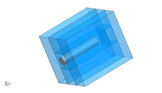
Figure 1: Part file containing both structure
and fluid volume

2.    
Create the Thermal/Flow FEM

Next, create the fem file. In the “Edit FEM” window, make sure to choose Simcenter Thermal/Flow (Flow) as the “Solver Environment”, as shown in Figure 2.

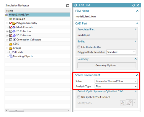
Figure 2: Creating the Thermal/Flow fem

Then create a 3D mesh for the air volume, as shown in Figure 3.

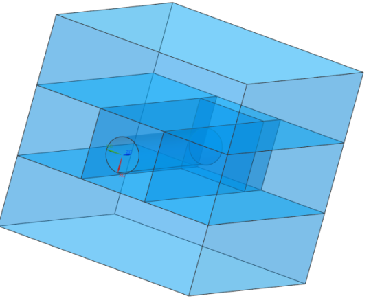
Figure 3: Mesh the air volume only. The
structure is not meshed.

3.    
Create the Flow Solution

We now create the “Simulation” file, and define a “Flow” analysis. As shown in Figure 4, define a non-turbulent transient analysis. Furthermore, in the “Result Options”, see Figure 5, check the “Pressure and Shear Resultants” box – these will be used for the mapping step.

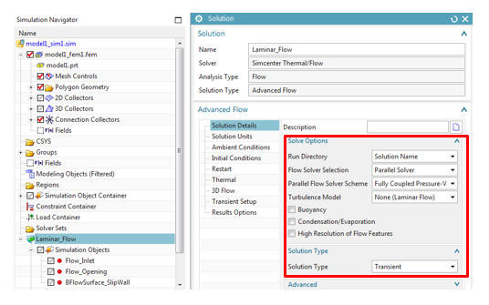
Figure 4: Flow Solution setup

Then, edit the “Transient Setup” tab as illustrated in Figure 5. 

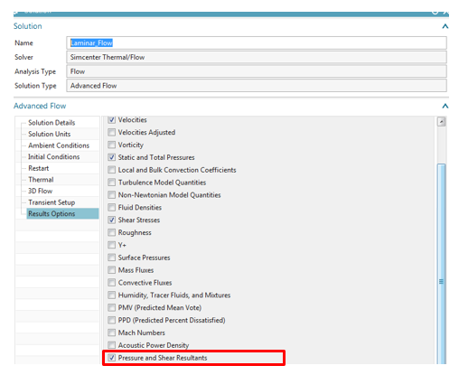
Figure 5: Results Options for flow forces

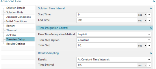
Figure 6:
Transient setup options

4.    
Apply the boundary conditions.

Three boundary conditions are applied:

• An inlet of 30 mm/sec at ambient conditions on the –Y faces.
• An opening at ambient conditions on the +Y faces.
• Slip walls to represent an extended fluid domain on the +X, -X and +Z faces.

As nothing is prescribed on the bottom surface, the solver automatically assumes no-slip, which represents a solid surface. Boundary conditions are shown in Figure 7.

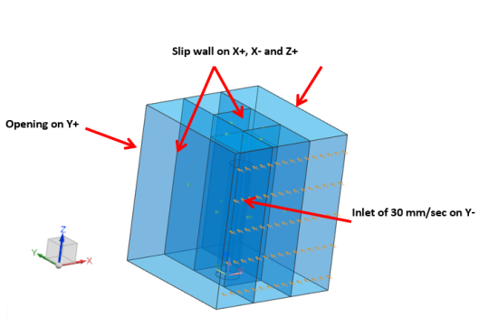
Figure 7: Boundary conditions

We now solve this Flow solution. An example of the flow velocity profiles is shown in Figure 8.

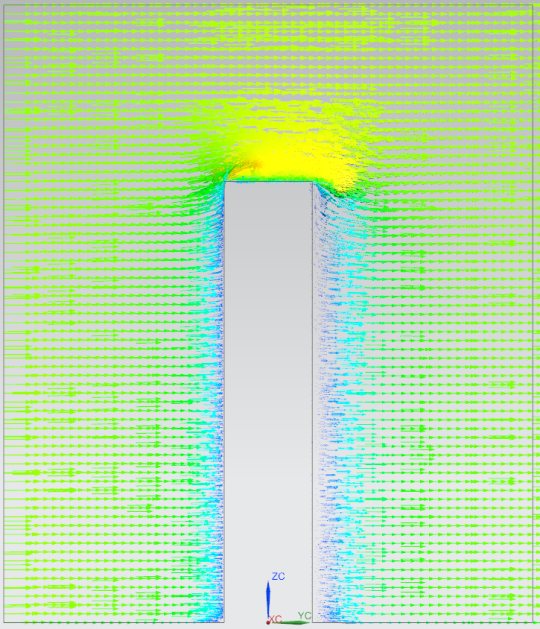
Figure 8: Flow velocity profile.

Mapping the flow forces

1.    
Create the structural mesh

Starting with the same part created in step 1, create a new fem file. In the “Edit FEM” window, make sure to choose the NX Nastran (Structural) “Solver Environment”, as shown in Figure 9.

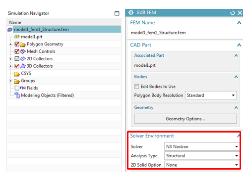
Figure 9: Creating the Structure fem

This time, we will only mesh the structure component and ignore the air volume. See Figure 10. An aluminum material is assigned to the tube.

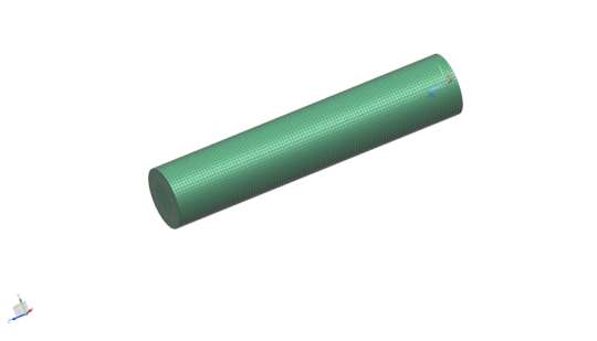
Figure 10: Structure mesh only. The air volume
is not meshed.

2.    
Create the Mapping Solution

To map the flow forces to the structural analysis, create a new “Simulation” file and choose a “Thermal-Flow” Solution with a “Mapping” type, as shown in Figure 11. If you leave the “Transient Times” table empty, the solver automatically selects all transient time steps from the flow solution.

Figure 11: Create a Mapping Solution

Next, in the “Optional Output” tab, check the boxes shown in Figure 12 to create the mapping and target Nastran structural solution. A static solution is created. This type of analysis is valid when inertial effects are negligible and where the dynamic content of the flow pressures is well separated from the structures principal modes.

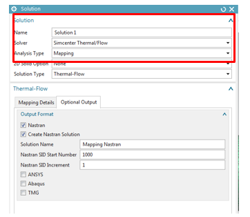
Figure 12: Creating the Mapping and Nastran Solution

3.    
Solve the Mapping Solution

Before solving the Mapping Solution, we define a “Mapping Target Set”. This defines the surfaces on which the flow forces will be mapped. Select the cylindrical face of the tube and its free face, as shown in Figure 13 and Figure 14. We can now solve the Mapping Solution. An example of the mapped forces at a given time step is shown in Figure 15.

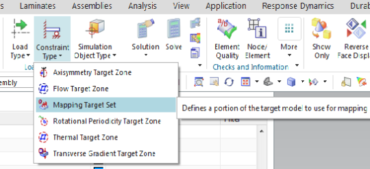
Figure 13: Mapping Target Set

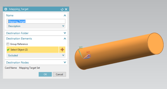
Figure 14: Select the mapped surfaces

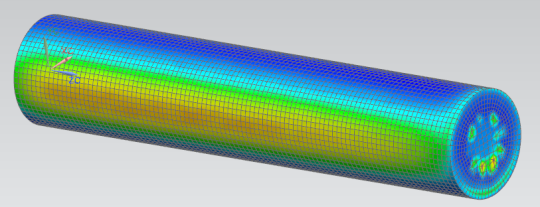
Figure 15: Example of mapped forces

4.    
Solve the structural solution

The “Simulation Navigator” now shows one subcase corresponding to each transient time step of the flow solution. See Figure 16.

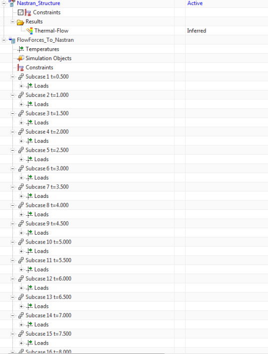
Figure 16: Subcase created for each transient
time step of the flow solution

Before solving, we fix the translational degrees of freedom on the –X face of the tube. Solve the solution.

5.    
View displacement results

Next, select a subcase and display the displacement results, as shown in Figure 17. The deformed structure is shown together with the undeformed mesh in Figure 18.

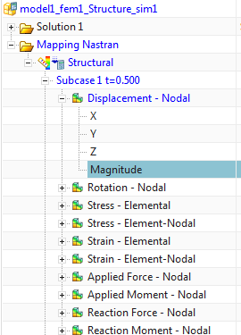
Figure 17: Nodal displacement results

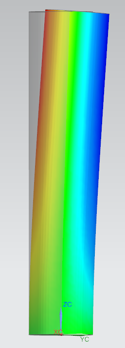
Figure 18: Deformed and undeformed structure