Quick Overview
This Tips & Trick shows how to use the Combined Load-cases functionality in NX, which allows you to create combinations of linear load case results, thereby avoiding the need to pre-define and solve all the required combinations.
Core content
Suppose you are performing a linear statics analysis on a model which will experience top, bottom and side loading. You’ve been asked to provide results for the following loading conditions:
- Top loading only
- Bottom loading only
- Side loading only
- Top and bottom loading
- Top and side loading
- Top, bottom, and side loading
You could define a solution with 6 different sub-cases. Alternatively, you can create a solution containing only 3 sub-cases, one for each individual load case, thereby generating a potentially much smaller results file. After you solve the model, you can use the Combined Load-cases command to create named, combined load cases representing each of the loading conditions.
Steps
In the sim navigator, create a static solution with 3 subcases, each one containing a single load set: Top load, bottom load and side load, respectively.
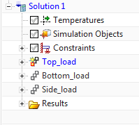
Figure 1. A static solution with 3 subcases
When the solution is complete, right click on the structural results node and select Combined Loadcases.
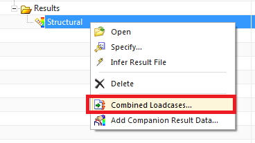
Figure 2. Defining combined load cases
In the Load Case Combine dialog, type a descriptive name for the load case combination: For example, Top and Side loading and then click Create. Select the load case to be included in the combination from the Load case component box, enter a scale factor and then click on Add/Edit. In the combined load case definition box, you will see the load case name preceded by the specified scale factor. Repeat the process to enter the other load cases required for the combined loading. In case you need to delete or edit the scale factor of an added load case, simply select the load case in the combined load case definition box, then apply the changes and click on Add/Edit to apply the changes.
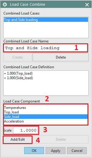
Figure 3. Defining load case combination
Clicking on OK generates the combined loading results that can be found in the Post Processing Navigator.
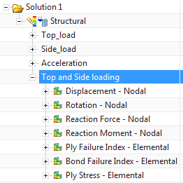
Figure 4. The result of the combined loads is added to the post processing navigator.
It is worth mentioning that prior to using the Combined Load-cases functionality; you should give some thought as to how you set up your analysis: Be sure to create a separate sub-case for each load case that you intend to combine. If you want to apply a scale factor, you may find it useful to define unit loads.
Other Example
As another example, assume you want to perform a linear static analysis including an external force applied to a lug as shown in Figure 5. Suppose that the results are required for multiple directions (θ=0,30,45,60,etc.) of the load, each with different magnitudes (F= F1, F2, F3, etc). You can create a solution with 2 sub-cases: The first sub-case will contain a horizontal unit load (u) and the second sub-case will contain a vertical unit load (v).
We know that F=|F| cos(θ) u+|F| sin(θ)v, where |F| is the magnitude of the applied load. Therefore, the results of the analysis under any load, F, can be simply obtained by combining the results of the 2 sub-cases with the scale factor of |F| cos(θ) for load u and a scale factor of |F| sin(θ) for load v. This method can be easily expanded for a force in 3D space.
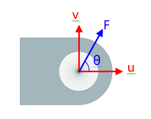
Figure 5. A load applied with a magnitude F at a direction θ.